Overview

• Embeddings map discrete or high-dimensional inputs into dense vectors that capture similarity and structure.
• Good embeddings make downstream learning easier by placing related items closer in vector space.
• This note summarises embeddings for text, images, audio, and structured data, plus practical tips.

Core Idea

• An embedding is a learnable function $f(x) \rightarrow \mathbb{R}^d$.
• Similar inputs should have nearby vectors (cosine similarity or dot product).
• Embeddings are usually trained jointly with a task or via self-supervision.

Sparse vs Dense Embeddings

Sparse Embeddings

• Most dimensions are zero; only a small subset are non-zero.
• Common examples: one-hot vectors, bag-of-words, and TF-IDF.
• Usually high-dimensional, such as vocabulary-sized vectors.
• Easy to interpret because each dimension maps to a specific token/feature.

Dense Embeddings

• Most dimensions contain non-zero values.
• Common examples: Word2Vec, GloVe, BERT token embeddings, CLIP embeddings.
• Usually lower-dimensional, such as $d=128$ to $d=4096$.
• Harder to interpret directly, but better at capturing semantic similarity.

Key Tradeoffs

• Interpretability:
  • Sparse vectors are more human-readable.
  • Dense vectors are less interpretable but often more expressive.
• Memory and compute:
  • Sparse vectors can be memory-heavy at very large vocab sizes.
  • Dense vectors are compact and efficient for neural models.
• Generalisation:
  • Sparse methods treat tokens as mostly independent.
  • Dense methods share statistical strength across similar tokens/items.
• Best use cases:
  • Sparse: classical IR/search baselines, small-data linear models.
  • Dense: semantic search, transfer learning, deep learning pipelines.

Practical Rule

• Start with sparse features (for example TF-IDF) for a fast baseline.
• Move to dense embeddings when you need semantic similarity, transfer, or multimodal alignment.

Text Embeddings

Tokenisation matters

• Word-level: simple but large vocab and OOV issues.
• Subword (BPE/WordPiece): handles OOV and morphology.
• Character: robust but longer sequences.

Static vs Contextual

• Static (Word2Vec, GloVe, fastText): one vector per token.
• Contextual (BERT, GPT-style): token vector depends on surrounding words.

Training objectives

• Skip-gram / CBOW: predict context words.
• Masked language modelling: predict masked tokens.
• Contrastive: pull positives together, push negatives apart.

Practical Notes

Default to cosine similarity for semantic comparisons

• Cosine similarity is usually a strong first choice for embedding search and clustering.

Normalize before cross-batch dot-product comparisons

• L2-normalization helps keep similarity scores stable across batches.

Use mean pooling as a sentence-level baseline

• Averaging token embeddings is a simple and often competitive first approach.

BPE (Byte-Pair Encoding)

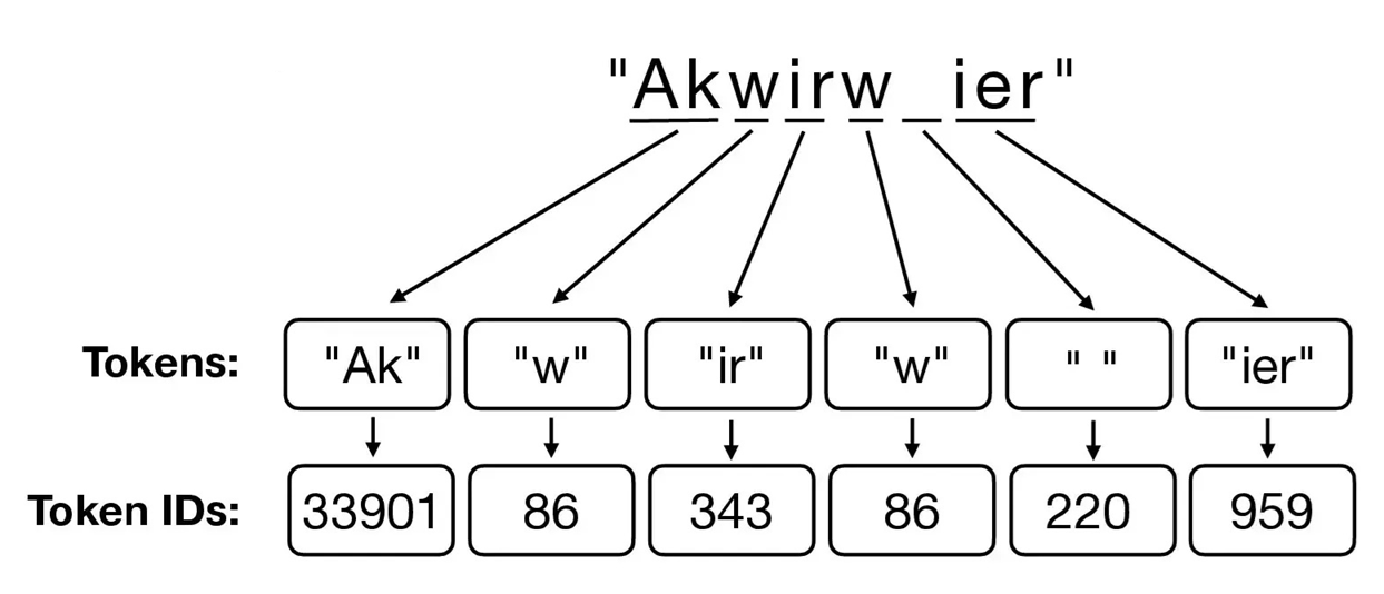
Core Idea

• Start with characters, then repeatedly merge the most frequent adjacent pairs.
• Why it works: frequent word fragments become subwords, so rare words can be built from pieces.

Steps

Step 1: Initialise the vocabulary

• Build an initial vocabulary of characters plus a word boundary marker.
• Represent each word as a sequence of characters.

Step 2: Count symbol pairs

• Scan the corpus and count all adjacent symbol pairs.
• Track the most frequent pairs across the full corpus.

Step 3: Merge the best pair

• Merge the most frequent pair into a new symbol.
• Add the new symbol to the vocabulary.

Step 4: Update the corpus

• Replace all occurrences of the merged pair.
• Recompute adjacent pairs on the updated corpus.

Step 5: Repeat until target size

• Loop steps 2–4 until you hit the vocabulary budget.
• Stop early if no merges are beneficial.

Step 6: Tokenise new text

• Apply the learned merges in order.
• Produce a sequence of subword tokens.

Strengths and Weaknesses

• Strengths:
  • Controls vocabulary size.
  • Handles OOV by breaking into subwords.
• Weaknesses:
  • Not probabilistic; merges are frequency-based only.
  • Can split words in unintuitive ways (e.g., im|port|ant).
• When to use: strong default for modern NLP and LLM tokenisers.

WordPiece

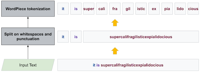
Core Idea

• Like BPE but merges maximise likelihood of the training data.
• Why it works: likelihood-driven merges favour subwords that explain the corpus well, so frequent patterns become stable tokens while rare words still decompose cleanly.

Steps

Step 1: Initialise the vocabulary

• Start with characters and word boundary markers.
• Represent each word as a sequence of characters.

Step 2: Score segmentations

• Train a simple language model to score candidate segmentations.
• Estimate likelihood for current token splits.

Step 3: Propose new subwords

• Consider adding candidate subwords.
• Measure likelihood improvement for each candidate.

Step 4: Add the best candidate

• Add the subword that yields the largest likelihood gain.
• Update the vocabulary.

Step 5: Re-tokenise the corpus

• Re-segment the corpus with the updated vocabulary.
• Recompute statistics for the next iteration.

Step 6: Repeat until target size

• Continue steps 2–5 until you hit the vocabulary budget.
• Stop early if gains are negligible.

Step 7: Tokenise new text

• Apply longest-match-first subword matching.
• Produce token sequences for the model.

Strengths and Weaknesses

• Strengths:
  • Often yields more linguistically coherent subwords.
  • Common in BERT-family tokenisers.
• Weaknesses:
  • Training is a bit more complex than BPE.
• When to use: transformer models where stable, reusable tokenisers matter.

TF-IDF

Core Idea

• Sparse vector for a document based on word frequency scaled by rarity.
• Why it works: common words get down-weighted and informative, rare terms are emphasised, making documents easier to separate.

Steps

Step 1: Build the vocabulary

• Extract terms from the corpus.
• Optionally remove stopwords or apply stemming.

Step 2: Compute term frequency

• For each document $d$, compute

• Use raw counts or log-scaled counts.
• Term frequency (TF):
  • Captures how frequent a term is within a document.
  • Higher TF suggests the term is more informative about that document.

Step 3: Compute document frequency

• Count how many documents contain each term $t$.
• Store $\text{df}(t)$ for the full corpus.
• Document frequency (DF):
  • $\text{df}(t)$ is the number of documents containing term $t$.
  • Rare terms (low $\text{df}$) help discriminate documents.

Step 4: Compute inverse document frequency

• $\text{idf}(t) = \log\frac{N}{\text{df}(t) + 1}$.
• Use smoothing to avoid division by zero.
• Inverse document frequency (IDF):
  • Terms appearing in every document get weight near 0.
  • This helps for discrimination based on unique-ness

Step 5: Build TF-IDF vectors

• $\text{tfidf}(t, d) = \text{tf}(t, d)\cdot \text{idf}(t)$.
• Assemble a sparse vector per document.

Step 6: Normalise (optional)

• L2-normalise vectors for cosine similarity.
• Keep raw values for some classifiers.

Strengths and Weaknesses

• What it captures: salience of words that are frequent in a document but rare overall.
• Strengths:
  • Fast, interpretable, strong baseline for retrieval and classification.
• Weaknesses:
  • Ignores word order and context.
  • High-dimensional and sparse.
• When to use: small/medium corpora, classical IR, or quick baselines.

Word2Vec

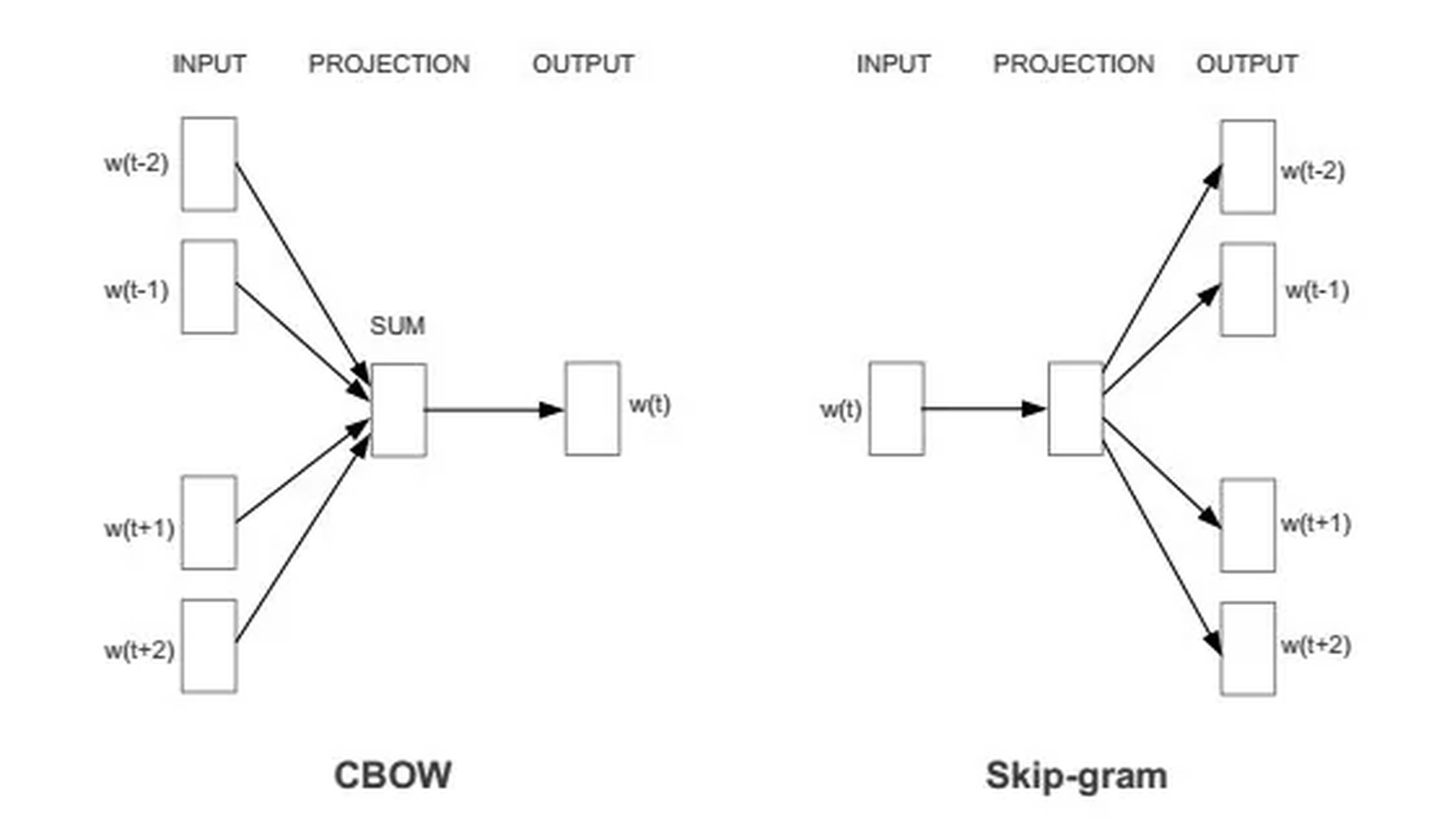
Core Idea

• Learn dense word vectors from local context.

Steps (CBOW)

Step 1: Build training pairs

• Slide a fixed window over text.
• Use the context words as input and the centre word as target.

Step 2: Predict the centre word

• Compute scores for all vocab terms.
• Apply a softmax to get probabilities.

Step 3: Update embeddings

• Increase the probability of the true centre word.
• Decrease probabilities for incorrect words.

Steps (Skip-gram)

Step 1: Build training pairs

• Slide a fixed window over text.
• Use the centre word as input and each context word as target.

Step 2: Predict context words

• Compute scores for context words.
• Optimise the sum of log-probabilities.
• Training tricks:
  • Negative sampling replaces full softmax with a few negative examples.
  • Subsampling frequent words improves rare word quality.

Strengths and Weaknesses

• Strengths:
  • Captures semantic similarity and analogies.
• Weaknesses:
  • One vector per word (no context).
  • Struggles with polysemy.
• When to use: quick static embeddings or as a baseline.

BERT (Contextual Embeddings)

Core Idea

• Bidirectional transformer trained with masked language modelling.
• Why it works: each token attends to both left and right context, yielding richer representations.

Steps (pretraining)

Pretraining Step 1: Prepare inputs

• Tokenise with WordPiece.
• Add special tokens ([CLS], [SEP]) and segment IDs.

Pretraining Step 2: Apply masking

• Randomly mask a subset of tokens (e.g., 15%).
• Replace some with [MASK], some with random tokens.

Pretraining Step 3: Encode with the transformer

• Feed the sequence into a bidirectional transformer.
• Produce contextual hidden states for all positions.

Pretraining Step 4: Predict masked tokens

• Use final hidden states to predict original tokens.
• Compute masked language modelling loss.

Pretraining Step 5: Optional NSP objective

• Predict whether sentence B follows sentence A.
• Used in original BERT, removed in later variants.

Pretraining Step 6: Optimise

• Update all weights to minimise total pretraining loss.

Steps (finetuning)

Finetuning Step 1: Add a task head

• Classification, span prediction, or tagging head.
• Use [CLS] or token-level embeddings as inputs.

Finetuning Step 2: Train on task data

• Feed labelled data through the model.
• Backpropagate task loss through all layers.

Finetuning Step 3: Tune for the task

• Use a smaller learning rate and fewer epochs.
• Optionally freeze lower layers for stability.

Strengths and Weaknesses

• Output: each token embedding depends on its full context.
• Strengths:
  • Strong transfer performance; good for classification, QA, NER.
• Weaknesses:
  • Heavier compute and memory.
  • Masked objective does not exactly match generation.
• When to use: contextual tasks where nuance matters and compute is available.

GPT-Style (Autoregressive) Encodings

Core Idea

• Unidirectional transformer trained to predict the next token.
• Why it works: next-token prediction forces the model to build rich, contextual representations.

Steps (pretraining)

Pretraining Step 1: Prepare inputs

• Tokenise text and build a causal attention mask.
• Use a fixed context window.

Pretraining Step 2: Predict next tokens

• For each position, predict the following token.
• Compute cross-entropy loss over the vocabulary.

Pretraining Step 3: Optimise

• Update all weights to minimise next-token loss.

Steps (finetuning)

Finetuning Step 1: Add task formatting

• Format prompts with instructions/examples.
• Optionally add a task head for classification.

Finetuning Step 2: Train on task data

• Optimise either supervised loss or instruction-tuned loss.

Strengths and Weaknesses

• Output: each token embedding depends on left context only.
• Strengths:
  • Strong for generation and long-form text.
  • Scales well with data and compute.
• Weaknesses:
  • No right context at training time.
  • Can be sensitive to prompting.
• When to use: generation, summarisation, open-ended tasks.

Positional Embeddings

• Models without recurrence need position information.

Why positions matter

• Self-attention is permutation-invariant: without positions, token order is lost.
• Position signals let the model distinguish “dog bites man” from “man bites dog”.

Absolute (Learned) Positions

• Idea: A lookup table where each index is a position embedding.
• How it works:
  • Add or concatenate position vectors to token embeddings.
  • Train position vectors jointly with the model.
• Pros: Simple and effective for fixed-length inputs.
• Cons: Does not extrapolate well beyond training length.

Sinusoidal Positions

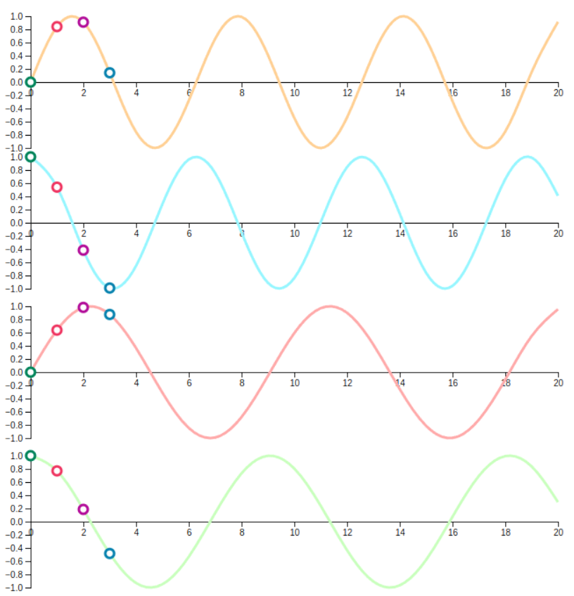
• Idea: Deterministic sine/cosine functions with different frequencies.
• How it works:
  • $\text{PE}_{(pos,2i)} = \sin(pos / 10000^{2i/d})$
  • $\text{PE}_{(pos,2i+1)} = \cos(pos / 10000^{2i/d})$
• Pros: No extra parameters; can extrapolate to longer sequences.
• Cons: Slightly less flexible than learned embeddings.

Relative Positions

• Idea: Encode distance between tokens instead of absolute index.
• How it works:
  • Modify attention scores based on relative offsets.
  • Bias attention toward nearer or specific relative positions.
• Pros: Generalises better to longer inputs; captures local patterns.
• Cons: More complex to implement; adds compute.

Rotary Positional Encoding (RoPE)

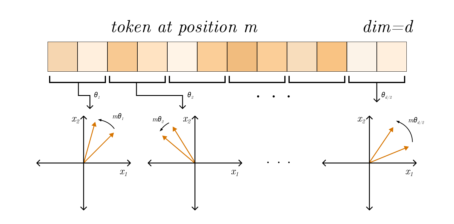
• Idea: rotate query/key vectors by a position-dependent angle.
• Why it works: turns relative position into a rotation in vector space.
• Pros: Strong performance and extrapolation in practice.
• Cons: More specialised; can be sensitive to scaling choices.
• 1D RoPE (for text):
  • Rotate each 2D pair in the embedding using the token position.
  • Use different frequencies per pair.
  • $\omega$ is a fixed frequency, not a trained parameter.
  • Each pair gets a different $\omega$ (often a geometric progression).

Practical Notes

Choose add vs concat based on model budget

• Adding positional signals keeps dimensionality fixed, while concatenation increases it.

Use learned 2D positions for ViT patch tokens

• Learned 2D positional embeddings are a common and effective default in vision transformers.

Prefer relative or RoPE-style methods for long context

• Relative/rotary schemes usually extrapolate better than basic absolute embeddings.

Image Embeddings

Common approaches

• CNN features: global average pooled activations.
• Vision Transformers: patch embedding + positional embeddings.
• CLIP-style: map images and text into a shared space.

CNN Feature Embeddings

• Idea: use intermediate or pooled CNN activations as image vectors.
• How it works:
  • Pass image through a pretrained CNN.
  • Take the last conv block features and apply global average pooling.
• See also: Pre-trained Vision Encoders
• Strengths:
  • Strong for textures and local patterns.
  • Works well with limited data via transfer learning.
• Weaknesses:
  • Limited global context vs transformers.
• When to use: fast baselines, small datasets, edge deployment.

Vision Transformer (ViT) Patch Embeddings

• Idea: split image into patches and treat each as a token.
• How it works:
  • Flatten $P \times P$ patches into vectors.
  • Project to embedding dimension and add positional embeddings.
  • Use the [CLS] token (or pooled tokens) as the image embedding.
• See also: Pre-trained Vision Encoders
• Strengths:
  • Captures global context well.
  • Scales with data and compute.
• Weaknesses:
  • Data-hungry without pretraining.
• When to use: large datasets or strong pretrained backbones.

CLIP-Style Multimodal Embeddings

• Idea: train image and text encoders to align in a shared space.
• How it works:
  • Encode images and captions.
  • Use contrastive loss to pull matching pairs together.
• Strengths:
  • Zero-shot classification and retrieval.
  • Flexible across domains with text prompts.
• Weaknesses:
  • Can be prompt-sensitive.
• When to use: retrieval, open-vocabulary classification, multimodal tasks.

CLIP (Step-by-Step)

Step 1: Build image-text pairs

• Collect paired data $(I_i, T_i)$ where each image has a matching caption/text.
• In each batch, matched pairs are positives; non-matching pairs act as negatives.

Step 2: Encode each modality

• Pass image $I_i$ through an image encoder (CNN or ViT) to get vector $u_i$.
• Pass text $T_i$ through a text encoder (Transformer) to get vector $v_i$.

Step 3: Project into shared space

• Map both outputs to the same embedding dimension with learned projection heads.
• L2-normalize vectors so cosine similarity is a dot product:

Step 4: Compute similarity matrix

• For a batch of size $N$, compute all image-text similarities:

• $\tau$ is a temperature parameter controlling softmax sharpness.

Step 5: Optimize contrastive loss

• Train with symmetric contrastive objectives:
  • image-to-text: image $i$ should match text $i$.
  • text-to-image: text $i$ should match image $i$.
• This pulls matched pairs together and pushes mismatched pairs apart.

Step 6: Use for inference

• Zero-shot classification: encode class prompts and pick the class with highest similarity to image embedding.
• Retrieval: nearest-neighbor search between image and text embeddings in shared space.

Self-Supervised Vision Embeddings

• Idea: learn embeddings without labels using pretext tasks.
• Methods:
  • Contrastive (SimCLR, MoCo).
  • Masked image modelling (MAE, BEiT).
• Strengths:
  • Strong transfer performance.
  • Reduces reliance on labels.
• When to use: label-scarce domains or foundation model pretraining.

Practical Notes

Start with linear probing for transfer setup

• Pretrained image encoders often perform strongly with a lightweight linear head.

Normalize embeddings for retrieval

• L2-normalization is typically required for stable nearest-neighbor similarity search.

Audio Embeddings

What the model sees (representations)

• Raw waveform: 1D signal at 16k/44.1k Hz. Preserves phase and fine timing.
• Spectrograms: 2D time-frequency grids via STFT.
• Log-mel spectrograms: compress frequency with mel filters and log amplitude. Strong default.
• MFCCs: decorrelated log-mel features; often used in classical pipelines.

Typical pipeline

• Frame the waveform into overlapping windows (e.g., 25 ms with 10 ms hop).
• Convert to frequency domain (STFT) and apply mel filterbank.
• Log-scale and optionally mean-variance normalise.
• Feed to encoder and pool to a fixed-length embedding.

Encoder families

• CNNs over spectrograms:
  • Treat time-frequency as an image.
  • Convolutions learn local patterns like harmonics and onsets.
  • Pooling reduces time/frequency resolution to build invariance.
• CRNNs (CNN + RNN):
  • CNN extracts local features, RNN aggregates temporal dynamics.
  • Good when sequence order matters (speech, music phrases).
• Transformers:
  • Use patching or strided convs to create tokens.
  • Self-attention captures long-range temporal structure.
• Waveform models:
  • 1D conv stacks or transformer encoders on raw audio.
  • Avoids hand-crafted features but needs more data.

Training objectives (how embeddings are learned)

• Supervised: classify speaker, instrument, genre, scene, keyword.
  • Embedding is taken from a pre-logit layer for transfer.
• Contrastive:
  • Pull together different augmentations of the same clip.
  • Push apart unrelated clips in a batch (InfoNCE-style).
• Self-supervised predictive:
  • Predict future frames or masked segments.
  • Forces the model to capture temporal structure.
• Metric learning:
  • Triplet loss for speaker verification or audio search.

Pooling to a fixed vector

• Mean / max pooling over time: fast and effective baseline.
• Attention pooling: learn weights for important frames.
• NetVLAD / statistic pooling: aggregate with richer summary stats.
• Pooling choice controls whether embeddings capture global content or salient moments.

Augmentations that matter

• Time shift / crop: robustness to alignment.
• Additive noise / reverb: robustness to environment.
• Time stretch / pitch shift: invariance to tempo or pitch.
• SpecAugment: time/frequency masking on spectrograms.

Practical Notes

Use a strong audio front-end baseline first

• Log-mel spectrograms at 16 kHz with 64-128 mel bins are a reliable default.

Keep normalization policy consistent

• Per-clip or per-dataset normalization can work, but train/inference mismatch hurts transfer.

Match embedding post-processing to objective

• Retrieval usually benefits from L2-normalized vectors; classification can work with raw embeddings.

Watch for shortcut features

• Background noise and microphone artifacts can leak label information and inflate metrics.

Evaluate robustness under domain shift

• Include out-of-domain and noisy benchmarks, not only in-domain test splits.

Structured Data Embeddings

Categorical features

• Use embedding tables instead of one-hot for large vocabularies.
• Rare categories can be bucketed into UNK.

Numerical features

• Standardise inputs before feeding into MLPs.
• Optionally embed via piecewise linear or bucket embeddings.

Mixed data

• Concatenate numerical features with categorical embeddings.
• Use feature crossing only when necessary to reduce complexity.

Graph Embeddings (Brief)

• Node embeddings via message passing (GCN, GAT).
• Graph-level embeddings via pooling (mean, sum, attention).
• Contrastive objectives work well for self-supervised graph learning.

How To Choose Embedding Size

• Too small: underfits, loses nuance.
• Too large: overfits, slower, harder to regularise.
• Rules of thumb:
  • Small vocab (<1k): 16–64 dims.
  • Medium (1k–100k): 64–256 dims.
  • Large (>100k): 256–1024 dims.
• Validate with downstream performance and memory budget.

Practical Tips

• Normalise for retrieval tasks; keep raw for classification unless needed.
• For nearest-neighbour search, use approximate indexes (FAISS, HNSW).
• Freeze vs finetune: freeze when data is small, finetune when domain shifts.
• Monitor for embedding collapse (all vectors become similar).

PyTorch Examples

import torch
import torch.nn as nn

# Token embeddings
tok_emb = nn.Embedding(num_embeddings=30000, embedding_dim=256)

# Positional embeddings (learned)
pos_emb = nn.Embedding(num_embeddings=512, embedding_dim=256)

# Categorical feature embedding
city_emb = nn.Embedding(num_embeddings=1000, embedding_dim=32)

# Simple sentence embedding: mean pooling
tokens = torch.randint(0, 30000, (8, 32))  # batch, seq
emb = tok_emb(tokens)
sent_emb = emb.mean(dim=1)